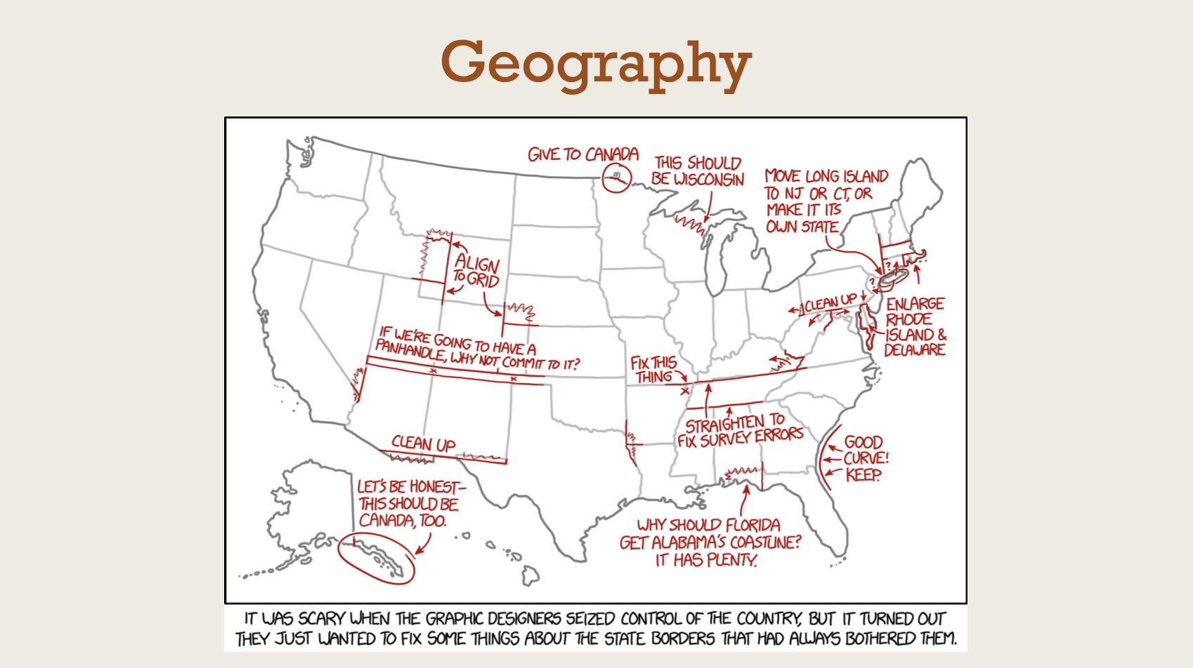
Geography
Materials for class on Tuesday, October 17, 2017
Contents
Slides
Download the slides from today’s lecture.
Creating maps with R
Download these shapefiles, unzip them, and put them in your data folder: 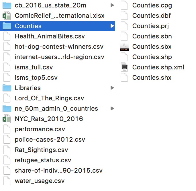
We’re going to make these two maps:
# Make sure you install the development version of ggplot with
# devtools::install_github("tidyverse/ggplot2")
library(tidyverse)
library(sf)
library(stringr)
library(gridExtra)

counties <- st_read("data/Counties/Counties.shp", quiet = TRUE)
libraries <- st_read("data/Libraries/Libraries.shp", quiet = TRUE)

libraries_county <- libraries %>%
  group_by(COUNTY) %>%
  summarize(num_libraries = n()) %>%
  mutate(NAME = str_to_upper(COUNTY))

counties_with_data <- counties %>%
  st_join(libraries_county) %>%
  mutate(people_per_library = POP_CURRES / num_libraries)

# In theory, geom_sf() should be able to plot points, and it does, but the
# latest development version ignores arguments like size = 5, so we have to use
# geom_point() instead. To do that, we have to extract the latitude and
# longitude values as individual columns, hence this libraries_lat_lon here
libraries_lat_lon <- cbind(libraries, st_coordinates(libraries))

plot_libraries <- ggplot() +
  geom_sf(data = counties_with_data, aes(fill = num_libraries), size = 0.25) +
  geom_point(data = libraries_lat_lon, aes(x = X, y = Y), size = 0.5) +
  scale_fill_gradient(low = "#fee0d2", high = "#de2d26", na.value = "white") +
  guides(size = FALSE,
         fill = guide_colorbar(title = "Number of libraries",
                               title.position = "top", barwidth = 10)) +
  coord_sf(crs = 26912, datum = NA) +
  theme_void() +
  theme(legend.position = "bottom")

plot_people <- ggplot() +
  geom_sf(data = counties_with_data, aes(fill = people_per_library), size = 0.25) +
  geom_point(data = libraries_lat_lon, aes(x = X, y = Y), size = 0.5) +
  scale_fill_gradient(low = "#fee0d2", high = "#de2d26", na.value = "white") +
  guides(size = FALSE,
         fill = guide_colorbar(title = "People per library",
                               title.position = "top", barwidth = 10)) +
  coord_sf(crs = 26912) +
  theme_void() +
  theme(legend.position = "bottom")

grid.arrange(plot_libraries, plot_people, nrow = 1)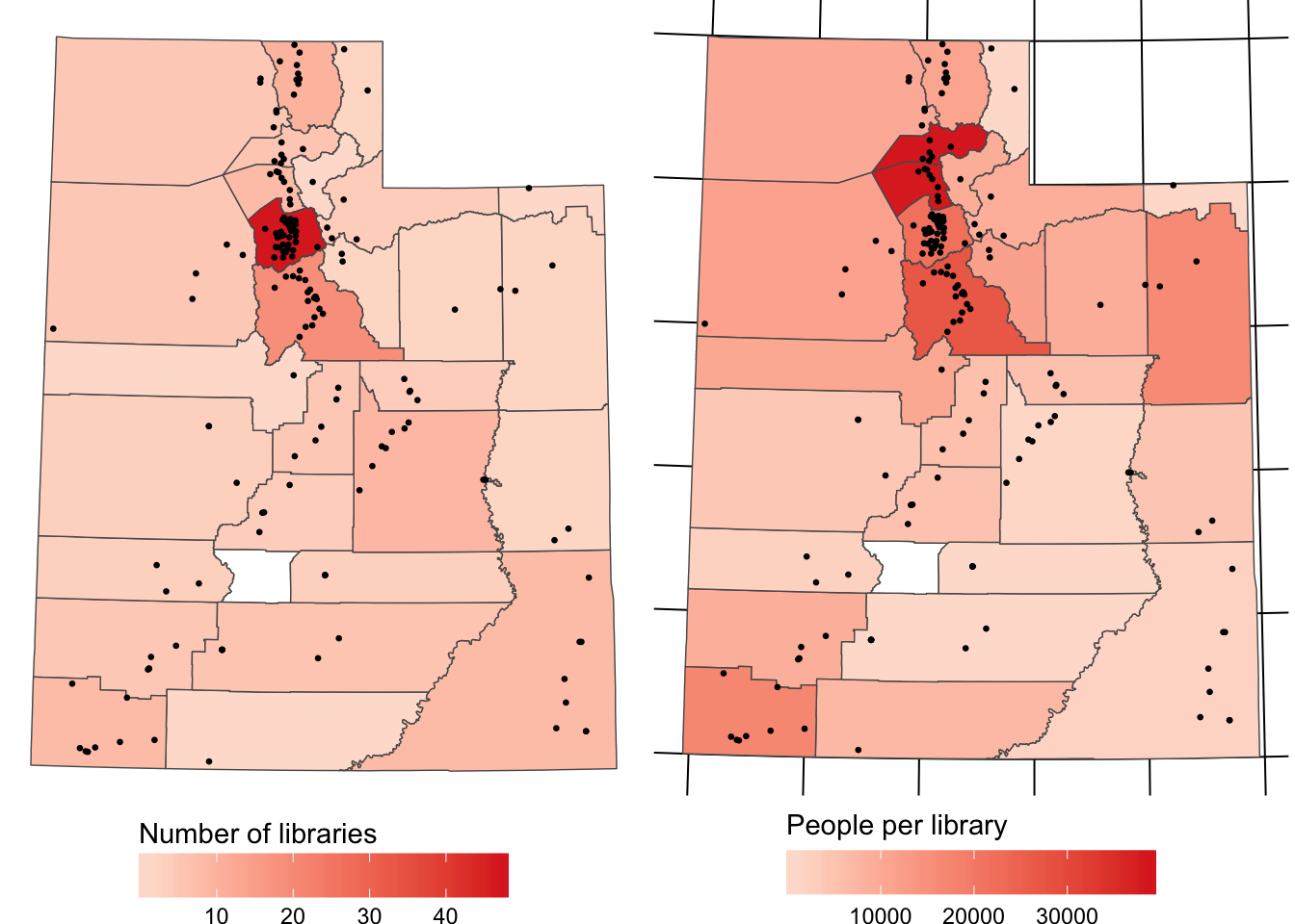
You’re on your own!
Find a story in this data on animal bites in Louisville. Summarize the data, make a plot in R, export it as a PDF, and enhance it in Illustrator or Inkscape.
See complete column descriptions. The data is released under a public domain license and hosted originally at Kaggle.
Louisville animal bites
Hint: You did stuff with this data last week, so you can refer to the code there. HOWEVER, don’t tell the same story this time. We already know about cat, dog, and other bites over time. Find a different story.
Feedback for today
Go to this form and answer these three questions (anonymously if you want):
- What new thing did you learn today?
- What was the most unclear thing about today?
- What was the most exciting thing you learned today?