Geography
Due by 11:59 PM on Monday, October 16, 2017
Complete these tasks in an R Markdown file and e-mail me a PDF of the final compiled document. Here’s the typical starter file. As always, I recommend saving it within an RStudio project. Make sure the final output is as clean and warning/message free as possible.
Task 1: Reflection memo
Write a 500-word memo about the assigned readings for this week. You can use some of the prompt questions there if you want:
- How can you know if a map projection is truthful or misleading?
- What’s wrong (or not wrong) with using points on maps? Choropleths? Lines?
As you write the memo, also consider these central questions:
- How do these readings connect to our main goal of discovering truth?
- How does what I just read apply to me?
- How can this be useful to me?
Task 2: Make a map
This task is not very code intensive—I’m giving you all the code!
That said, there’s still some work you have to do.
Step 1: Install extra software and R packages
- Plotting geographic stuff with ggplot is crazy easy nowadays with the new
sfpackage, which works nicely within the tidyverse paradigm. However, it’s so new that the CRAN version of ggplot doesn’t havegeom_sf()and other geographic plotting layers. You must install the development version of the package from GitHub. Doing this makes your computer compile the package from its source code and requires some fancy software to work.- If you’re using Windows, download and install Rtools (currently Rtools34.exe).
If you’re using macOS, open Terminal and type this:
A software update popup window should appear that will ask if you want to install command line developer tools. Click on “Install” (you don’t need to click on “Get Xcode”)xcode-select --install
Once you install those tools, make sure you install the
devtoolspackage in R (using the “Packages” panel, like normal), and then run this in your R console:
This will download, compile, and install the latest development version of ggplot. It’ll take a while—go eat something.devtools::install_github("tidyverse/ggplot2")- Using the “Packages” panel in RStudio, install these packages:
sf,maps,maptools, andrgeos - Final step for macOS people only: R doesn’t do all the geographic calculations by itself—it relies on a few pieces of standalone software behind the scenes. When people on Windows install
sf, those pieces of software should be installed automatically. This doesn’t happen on macOS, so you have to install them manually. The easiest way to do this is with Terminal. Here’s what you have to do:- Open Terminal
- If you haven’t already, go to brew.sh, copy the big long command under “Install Homebrew” (starts with
/usr/bin/ruby -e "$(curl -fsSL...), paste it into Terminal, and press enter. This installs Homebrew, which is special software that lets you install Unix-y programs from the terminal. You can install stuff like MySQL, Python, Apache, and even R if you want; there’s a full list of Homebrew formulae here.
Type this line in Terminal to install
gdal,geos, andproj:brew install gdal geos projWait for a few minutes—go eat something else.
Step 2: Actually make a map
In last week’s assignment, you looked at the percentage of different countries’ populations with access to the internet. This week, you’ll use the same data to map the level of internet access around the world in 2015.
I provide a full working example for you. Rather than just copying and pasting the code and knitting, though, I want you to run each line in RStudio and see what’s going on. In the starter Rmd file, I’ve included a list of code pieces you need to explain.
You need this data:
- Again, this data comes from Max Roser’s Our World in Data project.
Share of individuals using the internet, 1990-2015 - 1:50m cultural shapefiles from Natural Earth: Click on “Download countries” under “Admin 0 — Countries”, unzip the file, and put the whole folder in your data folder (so you should have something like this:
data/ne_50m_admin_0_countries/files.whatever)
The only strange, arcane thing in the code is coord_sf(crs = st_crs(XXXX)). This changes the coordinate system (or projection) for the map.TECHNICALLY coordinate systems and projection systems are different things, but I’m not a geographer and I don’t care that much about the nuance.
Recall from your reading that there are lots of different ways to project maps onto a flat surface. “CRS” refers to “coordinate reference system” and lets you specify a projection. There are standard indexes of more than 4,000 of these projections (!!!) at spatialreference.org. Here are some common ones:
- 54002: Equidistant cylindrical projection for the worldThis is essentially the Gall-Peters projection from the West Wing clip.
- 54004: Mercator projection for the world
- 54008: Sinusoidal projection for the world
- 54009: Mollweide projection for the world
- 54030: Robinson projection for the worldThis is my favorite world projection.
- 4326: WGS 84: DOD GPS coordinates (standard -180 to 180 system)
- 4269: NAD 83: Relatively common projection for North America
- 102003: Albers projection specifically for the contiguous United States
Alternatively, instead of using these index numbers, you can use any of the names listed at proj.4, such as:
st_crs("+proj=merc"): Mercator"+proj=robin": Robinson"+proj=moll": Mollweide"+proj=aeqd": Azimuthal Equidistant"+proj=cass": Cassini-Soldner
Here we go! First we load the internet users data:
# Install the most recent development version of ggplot from GitHub
# devtools::install_github("tidyverse/ggplot2")
library(tidyverse)
library(sf)

internet_users <- read_csv("data/share-of-individuals-using-the-internet-1990-2015.csv") %>%
  rename(users = `Individuals using the Internet (% of population) (% of population)`,
         iso_a3 = Code)

users_2015 <- internet_users %>%
  filter(Year == 2015)
Then we load the geographic data and combine it with the internet data:
world_shapes <- st_read("data/ne_50m_admin_0_countries/ne_50m_admin_0_countries.shp",
                        stringsAsFactors = FALSE)
## Reading layer `ne_50m_admin_0_countries' from data source `/Users/andrew/Sites/sites/dataviz/static/data/ne_50m_admin_0_countries/ne_50m_admin_0_countries.shp' using driver `ESRI Shapefile'
## Simple feature collection with 241 features and 63 fields
## geometry type: MULTIPOLYGON
## dimension: XY
## bbox: xmin: -180 ymin: -89.99893 xmax: 180 ymax: 83.59961
## epsg (SRID): 4326
## proj4string: +proj=longlat +datum=WGS84 +no_defs# left_join takes two data frames and combines them, based on a shared column
# (in this case iso_a3)
users_map <- world_shapes %>%
left_join(users_2015, by = "iso_a3") %>%
filter(iso_a3 != "ATA") # No internet in Antarctica. Sorry penguins.Finally, we plot the map:
pretty_map <- ggplot(users_map) +
  geom_sf(aes(fill = users), color = NA) +
  coord_sf(crs = st_crs(54030), datum = NA) +
  scale_fill_gradient(low = "#e7e1ef", high = "#dd1c77", na.value = "grey70",
                      limits = c(0, 100)) +
  guides(fill = guide_colorbar(title.position = "top",
                               title.hjust = "0.5",
                               title = "% of population",
                               barwidth = 10, barheight = 0.5)) +
  theme_void() +
  theme(legend.position = "bottom")

pretty_map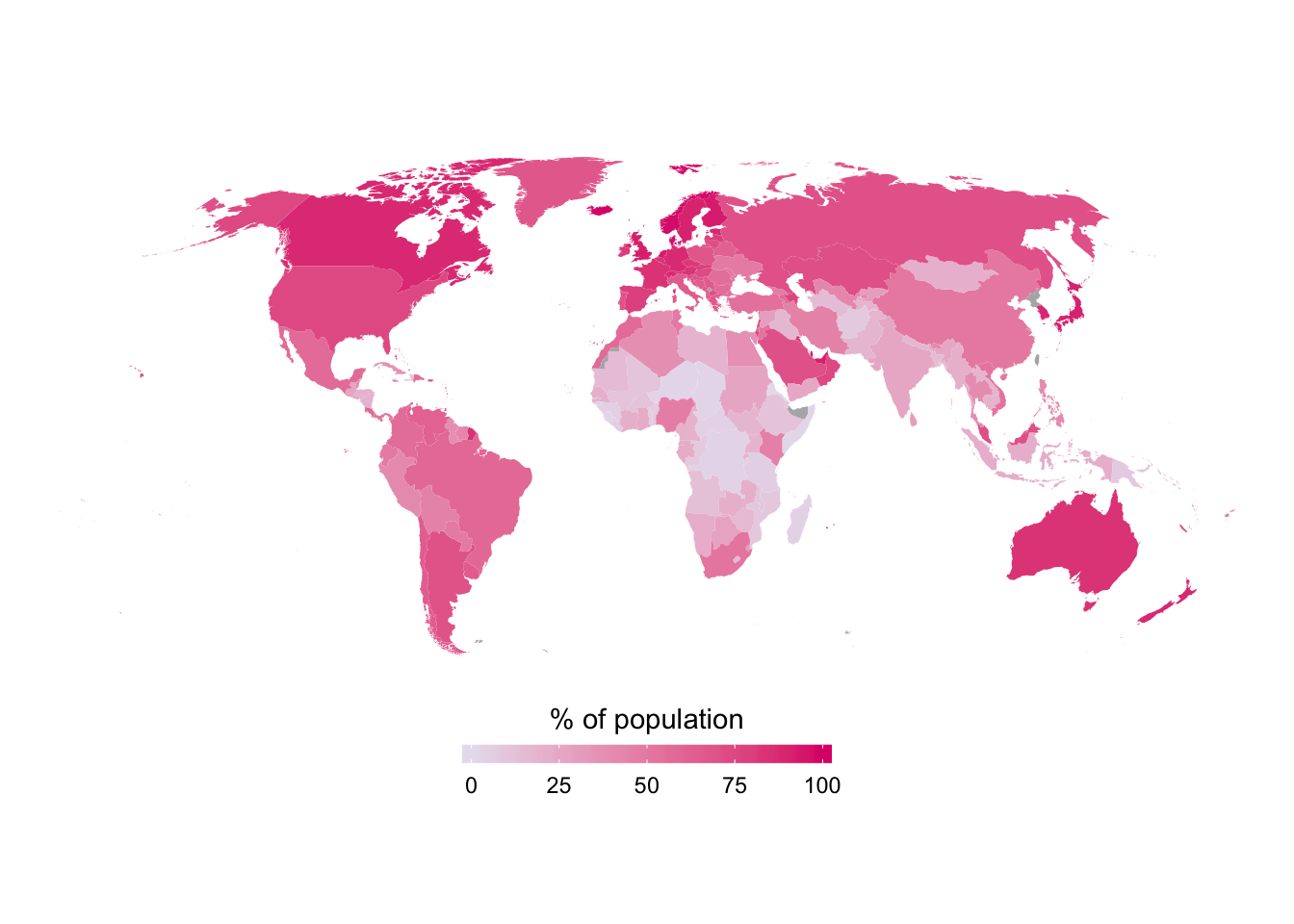
Task 3: Illustrator introduction
Step 1: Quickly get familiar with Illustrator (or Inkscape)
Watch and work through these tutorials (you can speed them up to 1.5× or 2× if you want):
- Set up a new document
- Get to know Illustrator
- Create and edit shapes
- Add text to your designs
- Organize content with layers
- Share artwork
These are all specific to Illustrator, but the same principles apply to Inkscape (though tools and options will have different names). I recommend learning Illustrator now while you have free access to it, and then in the future when you won’t necessarily have access to Adobe’s Creative Cloud, you’ll be able to translate your skills to Inkscape.
Step 2: Make something with Illustrator
- Use
ggsave()to save your map of internet users as a PDF. - Place the map in a new document in Illustrator.
- Enhance it with annotations, lines, shapes, etc. Make it fancy. But also follow the principles of CRAP and don’t go crazy.
- Export the completed graphic as a PDF and PNG.