Surveys and qualitative data
Materials for class on Tuesday, October 24, 2017
Contents
Slides
Download the slides from today’s lecture.
Text analysis and visualization
We can download any book from Project Gutenberg with gutenbergr::gutenberg_download(). The gutenberg_id argument is the ID for the book, found in the URL for the book. In class we looked at Anne of Green Gables, which has an ID of 45.
Once we’ve downloaded the book, we can tokenize the text (i.e. divide into words), and then create a long tidy data frame. tidytext does simple tokenization—it will not determine parts of speech or anything fancy like that. Look at the cleanNLP package for a tidy way to get full-blown natural language processing into R.
tidy_book <- book %>%
  mutate(line = row_number()) %>%
  unnest_tokens(word, text)

tidy_book %>% head() %>% knitr::kable()| gutenberg_id | line | word |
|---|---|---|
| 45 | 1 | anne |
| 45 | 1 | of |
| 45 | 1 | green |
| 45 | 1 | gables |
| 45 | 3 | by |
| 45 | 3 | lucy |
Word frequencies
We can filter out common stopwords and then view the 20 most frequent words:
plot_words <- tidy_book %>%
  anti_join(stop_words, by = "word") %>%
  count(word, sort = TRUE) %>%
  top_n(20, n) %>%
  mutate(word = fct_rev(fct_inorder(word, ordered = TRUE)))

ggplot(plot_words, aes(x = word, y = n)) +
  geom_col() +
  coord_flip()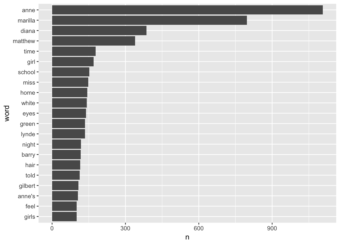
Sentiment analysis
There are several existing dictionaries of word sentiments, such as AFINN and Bing, which work differently—some use a continuous scale of negativity-positivity, whil others use a dichotomous variable:
| word | score |
|---|---|
| abandon | -2 |
| abandoned | -2 |
| abandons | -2 |
| abducted | -2 |
| abduction | -2 |
| abductions | -2 |
| word | sentiment |
|---|---|
| 2-faced | negative |
| 2-faces | negative |
| a+ | positive |
| abnormal | negative |
| abolish | negative |
| abominable | negative |
We can join one of these sentiment dictionaries to the list of words and find the most common positive and negative words:
plot_sentiment <- tidy_book %>%
  inner_join(get_sentiments("bing"), by = "word") %>%
  count(sentiment, word, sort = TRUE) %>%
  group_by(sentiment) %>%
  top_n(10, n) %>%
  ungroup() %>%
  arrange(sentiment, n) %>%
  mutate(word = fct_inorder(word))

ggplot(plot_sentiment, aes(x = word, y = n)) +
  geom_col() +
  coord_flip() +
  facet_wrap(~ sentiment, scales = "free")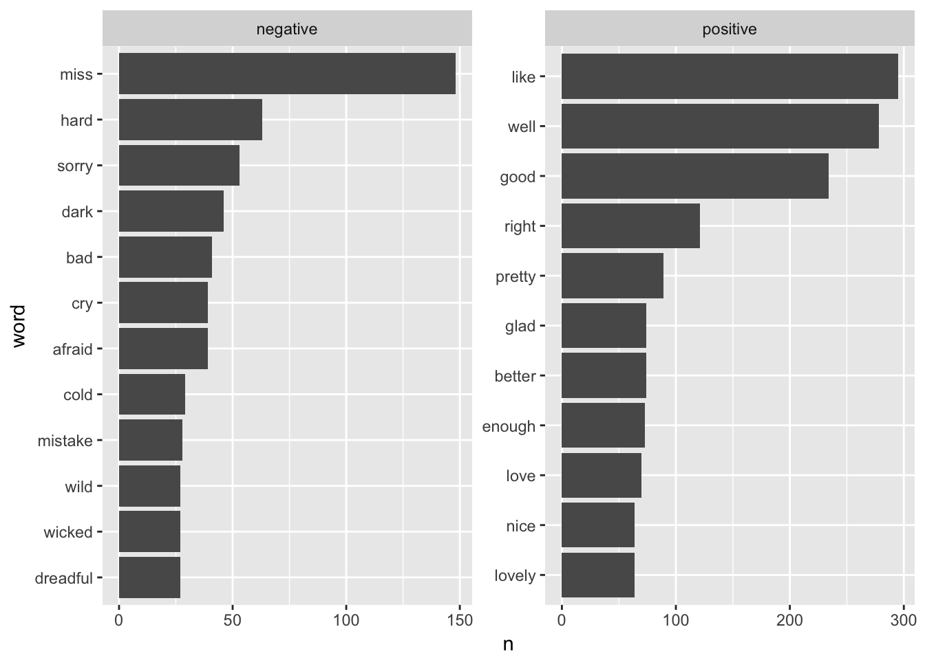
tf-idf: term frequency—inverse document frequency
Calculating the tf-idf lets us find the most unique words in individual documents in a collection, relative to other documents in the collection. Here we download four Dickens novels (A Tale of Two Cities (98), David Copperfield (766), Great Expectations (1400), and A Christmas Carol (19337)) and combine them into a tidy corpus:
We can then calculate the tf-idf across the different books:
dickens_tidy <- dickens %>%
  unnest_tokens(word, text) %>%
  count(title, word, sort = TRUE)

dickens_unique <- dickens_tidy %>%
  bind_tf_idf(word, title, n)

unique_top_10 <- dickens_unique %>%
  group_by(title) %>%
  top_n(10, tf_idf) %>%
  ungroup() %>%
  arrange(title, tf_idf) %>%
  mutate(word = fct_inorder(word))

unique_top_10 %>% head() %>% knitr::kable()| title | word | n | tf | idf | tf_idf |
|---|---|---|---|---|---|
| A Christmas Carol | cratchits | 14 | 0.0004730 | 1.386294 | 0.0006557 |
| A Christmas Carol | jacob | 16 | 0.0005406 | 1.386294 | 0.0007494 |
| A Christmas Carol | marley’s | 16 | 0.0005406 | 1.386294 | 0.0007494 |
| A Christmas Carol | fezziwig | 18 | 0.0006081 | 1.386294 | 0.0008430 |
| A Christmas Carol | marley | 20 | 0.0006757 | 1.386294 | 0.0009367 |
| A Christmas Carol | tim | 24 | 0.0008108 | 1.386294 | 0.0011241 |
ggplot(unique_top_10, aes(x = word, y = tf_idf, fill = title)) +
  geom_col(show.legend = FALSE) +
  coord_flip() +
  facet_wrap(~ title, scales = "free")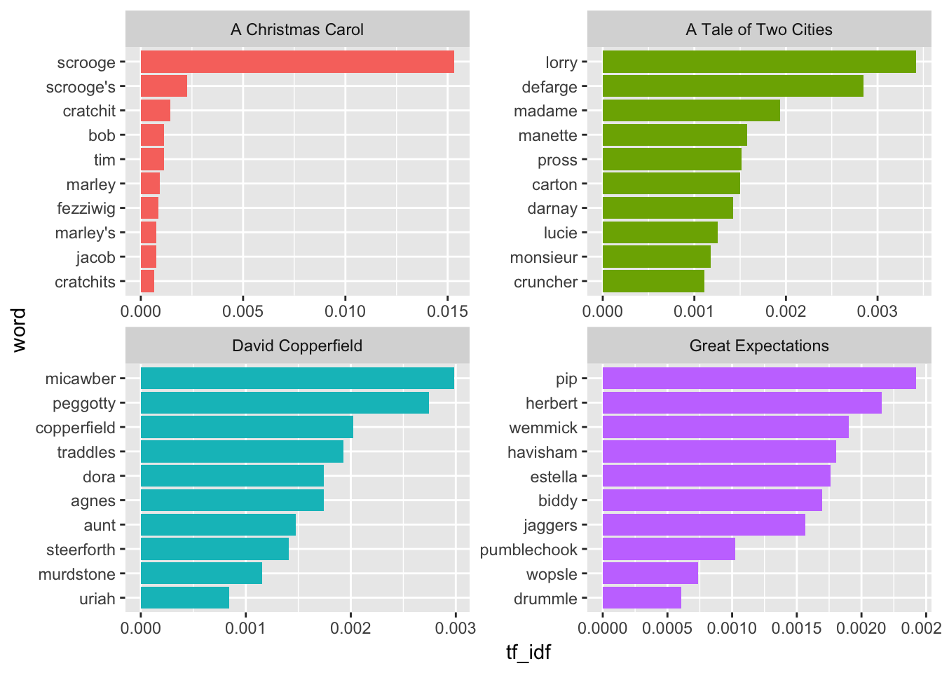
n-grams
We can also find the most common pairs of words, or n-grams. Rather than tokenizing by word, we can tokenize by ngram and specify the number of words—here we want bigrams, so we specify n = 2.
dickens_bigrams <- dickens %>%
  unnest_tokens(bigram, text, token = "ngrams", n = 2) %>%
  count(bigram, sort = TRUE)

dickens_bigrams %>% head() %>% knitr::kable()| bigram | n |
|---|---|
| of the | 3261 |
| in the | 3226 |
| it was | 1756 |
| to be | 1643 |
| that i | 1641 |
| to the | 1633 |
In class, we were interested in seeing which words are more likely to appear after “he” and “she” to see if there are any gendered patterns in Dickens’ novels (similar to this and this). To do this, we separate the bigram column into two columns named word1 and word2, and filter the data so that it only includes rows where word1 is “he” or “she”.
We then calculate the log odds for each pair of words to see which ones are more likely to appear across genders. We finally sort the data by the absolute value of the log ratio (since some are negative) and take the top 15.
dickens_bigrams <- dickens_bigrams %>%
  separate(bigram, c("word1", "word2"), sep = " ") %>%
  filter(word1 %in% c("he", "she")) %>%
  count(word1, word2, wt = n, sort = TRUE) %>%
  rename(total = nn)

dickens_ratios <- dickens_bigrams %>%
  group_by(word2) %>%
  filter(sum(total) > 10) %>%
  ungroup() %>%
  spread(word1, total, fill = 0) %>%
  mutate(logratio = log2(she / he)) %>%
  arrange(desc(logratio))

plot_ratios <- dickens_ratios %>%
  mutate(abslogratio = abs(logratio)) %>%
  group_by(logratio < 0) %>%
  top_n(15, abslogratio) %>%
  ungroup() %>%
  arrange(desc(logratio)) %>%
  mutate(word2 = fct_inorder(word2, ordered = TRUE))

ggplot(plot_ratios, aes(x = word2, y = logratio, color = logratio < 0)) +
  geom_pointrange(aes(ymin = 0, ymax = logratio), size = 0.5, fatten = 6) +
  coord_flip()
Feedback for today
First, make sure you fill out BYU’s official ratings for this class sometime before Saturday, October 28.
Second, go to this form and answer these questions (anonymously if you want):
- What were the two most important things you learned in this class?
- What were the two most exciting things you learned in this class?
- What were the two most difficult things you had to do in this class?
- Which class sessions were most helpful? Which were least helpful?
- Which readings were most helpful? Which were least helpful?
- What should I remove from future versions of this class?
- What should I add to future versions of this class?
- What else should I change in future versions of this class?
- Any other comments?