Comparisons
Materials for class on Tuesday, October 3, 2017
Contents
Slides
Download the slides from today’s lecture.
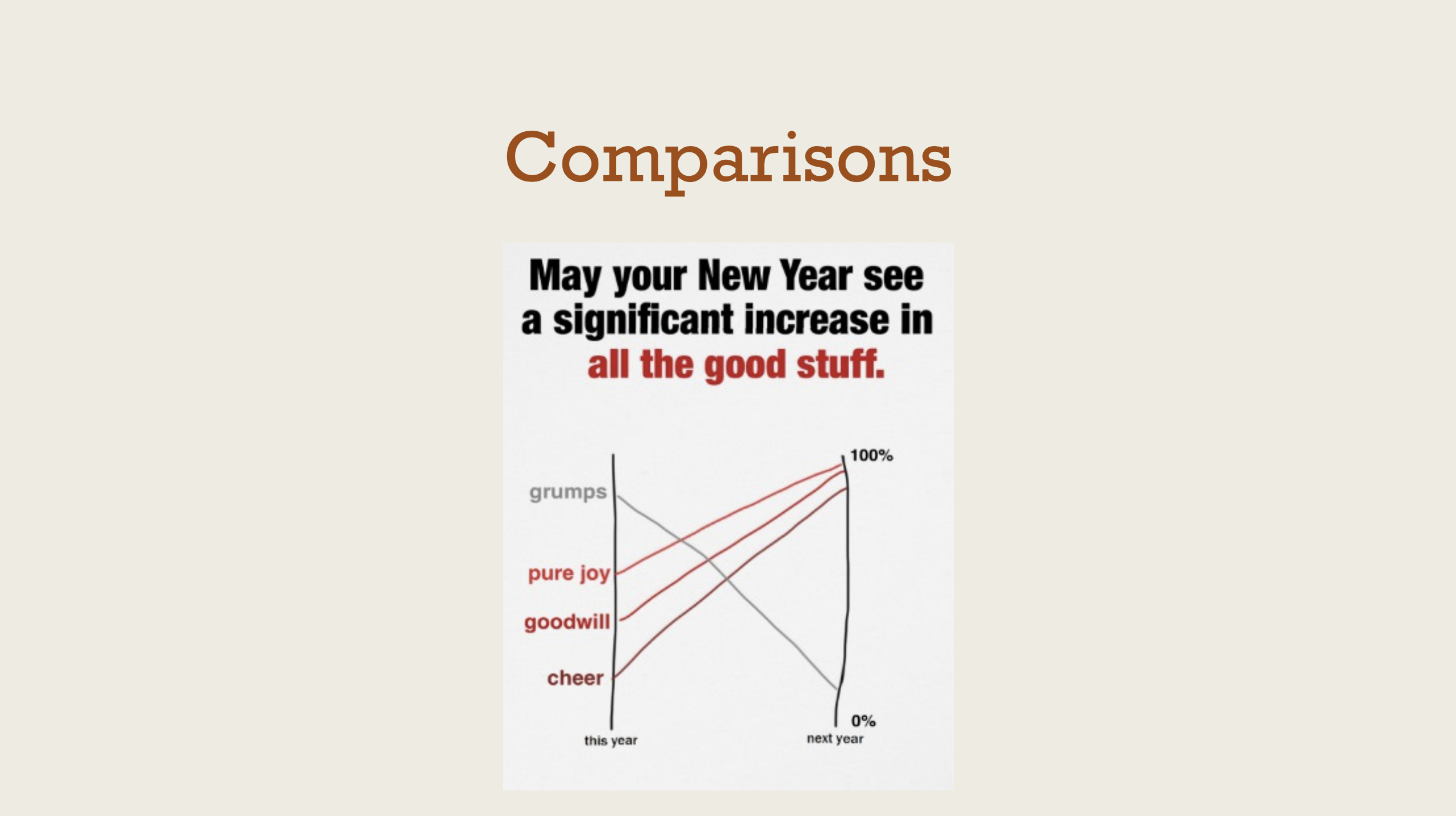
Comparing things
Sparklines
- Create in Excel
- Create in Word, HTML, and Adobe products with AtF Spark
- Create in R by saving really really tiny PDFs or PNGs
Small multiples
- Create in R with facets
Lollipops
Download Lord of the Rings data
First, we load the libraries we’ll need for all the examples. We’ll use tidyverse in both; we’ll use forcats in the lollipop chart and ggrepel in the slopegraph.
We load the CSV file into R and save it as a variable, or an object, named lotr. We use fct_inorder() inside a mutate command to make the Film variable an ordered factor so that the films plot in the correct order.
Next we summarize the data by race and gender. We can output the summarized table as a Markdown table with knitr::kable(). Remember that this syntax means that we’re using the kable() function inside the knitr package without actually loading it. Alternatively, you can run library(knitr) to load the package and then use kable() as needed without the double colon ::.
race_gender <- lotr %>%
  group_by(Race, Gender) %>%
  summarize(total_words = sum(Words))

knitr::kable(race_gender)| Race | Gender | total_words |
|---|---|---|
| Elf | Female | 1743 |
| Elf | Male | 1994 |
| Hobbit | Female | 16 |
| Hobbit | Male | 8780 |
| Man | Female | 669 |
| Man | Male | 8043 |
We can plot this summarized data, mapping variables to different aesthetics in the plot. A few things to note:
geom_pointrange()is what makes the lollipops. It takes two aesthetics:yminandymax. Here we wantyminto be zero so that all the lines start at the axis, but in other situations you could set it to an actual variable.position_dodge()andwidthis what tells the point ranges to be plotted side-by-side.coord_flip()rotates the whole plot so that the x-axis becomes the y-axis and vice versa. Alternatively, you can avoid usingcoord_flip()by usinggeom_pointrangeh()(and all the other*hfunctions likegeom_barhandgeom_colh()in theggstancelibrary.
ggplot(race_gender, aes(x = Gender, y = total_words, color = Race)) +
  geom_pointrange(aes(ymin = 0, ymax = total_words),
                  position = position_dodge(width = 0.5)) +
  coord_flip() +
  labs(x = NULL) +
  theme(legend.position = "bottom") +
  scale_color_manual(values = c("red", "orange", "blue"))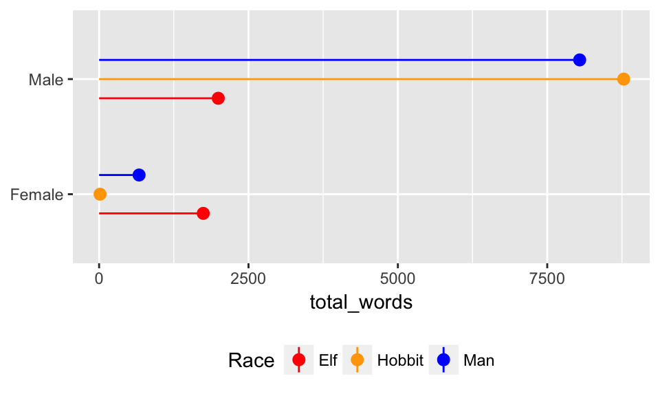
We can also plot race and gender across the three films. Because we used fct_inorder() earlier, the Film variable/column is an ordered factor and the films should be in order. Here we use the original lotr data frame instead of the summarized one, since we want the Film column too. We facet by film with facet_wrap(~ Film).
ggplot(lotr, aes(x = Gender, y = Words, color = Race)) +
  geom_pointrange(aes(ymin = 0, ymax = Words),
                  position = position_dodge(width = 0.5)) +
  coord_flip() +
  labs(x = NULL) +
  theme_light() +
  theme(legend.position = "bottom") +
  scale_color_manual(values = c("red", "orange", "blue")) +
  facet_wrap(~ Film)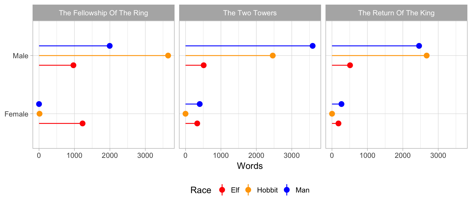
Slopegraphs
Download General Conference “isms” data This data comes from BYU’s LDS General Conference Corpus. I created a list of "*ism" divided between the 1950s/60s and the 1990s/2000s, and then copied/pasted the results in to a CSV file.
First, we load the data. I already filtered and summarized and tidyified this data, based on the original data that looked liked this. You can see the R code I used to clean and tidy the data here.
| word | decade | count | permil |
|---|---|---|---|
| Baptism | coldwar | 596 | 191.7 |
| Baptism | today | 609 | 207.8 |
| Communism | coldwar | 216 | 69.5 |
| Communism | today | 1 | 0.3 |
| Criticism | coldwar | 75 | 24.1 |
| Criticism | today | 51 | 17.4 |
| Mormonism | coldwar | 135 | 43.4 |
| Mormonism | today | 39 | 13.3 |
| Socialism | coldwar | 82 | 26.4 |
| Socialism | today | 0 | 0.0 |
Just plotting the data as-is gives us a rudimentary and ugly slopegraph. Note the group aesthetic—without it, the lines will not plot across the coldwar and today columns.
ggplot(isms, aes(x = decade, y = permil, group = word)) +
  geom_line(size = 1.5) +
  geom_text(aes(label = word))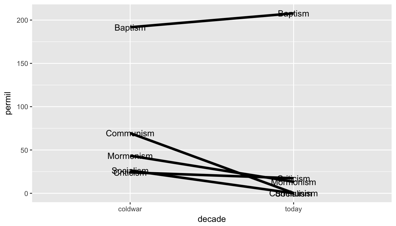
We can add a bunch of columns to the original isms data frame to help with plotting. Here’s what’s happening:
- We create a
label_firstvariable for the labels on the right side of the plot. We useifelse()—if the decade iscoldwar, usepaste0()to combine thewordcolumn with thepermil(or per million words) value, surrounded by parentheses; if it’s notcoldwar, use a missing value, orNA - We create a
label_lastvariable similarly, but this time only include thepermilvalue on rows that aren’tcoldwar - We create a
highlightcolumn to mark which lines we want colored - We recode the
decadecolumn to nicer values
isms_plot <- isms %>%
  mutate(label_first =
           ifelse(decade == "coldwar", paste0(word, " (", permil, ")"), NA)) %>%
  mutate(label_last = ifelse(decade == "today", permil, NA)) %>%
  mutate(highlight = ifelse(word %in% c("Socialism", "Communism"), TRUE, FALSE)) %>%
  mutate(decade = recode(decade,
                         coldwar = "1950-1969",
                         today = "1990-2009"))
We can use this enhanced data frame to add labels and color specific lines. Here’s the complete, final plot. A few things to note:
geom_text_repel()comes from theggrepellibrary and uses fancy algorithms to ensure labels don’t overlap. We setdirection = "y"to make sure the algorithm only shifts labels up and down (without it, the labels will show up everywhere), and we usenudge_xto move the labels horizontally away from the lines. We can useseed = some_numberto ensure the random positioning of the labels is the same each time the plot is generated.- We use a super minimal
theme_minimal()theme and them make a few more adjustments withtheme()to remove grid lines and the y axis text. - R will give two warnings saying
Removed 5 rows containing missing values (geom_text_repel).This is because it’s trying to plot missing values for the labels—but recall that we created those missing values in bothlabel_firstandlabel_last, so it’s not an issue. We’re purposely causing the warning and we can ignore it.
fancy_plot <- ggplot(isms_plot, aes(x = decade, y = permil, group = word, color = highlight)) +
  geom_point() +
  geom_line(size = 1.5) +
  geom_text_repel(aes(label = label_first), direction = "y", nudge_x = -1, seed = 1234) +
  geom_text_repel(aes(label = label_last), direction = "y", nudge_x = 1, seed = 1234) +
  scale_color_manual(values = c("black", "red")) +
  guides(color = FALSE) +
  labs(title = "Frequency of words ending in ‘ism’ in\nLDS General Conference talks",
       subtitle = "Word (occurrences per million words)",
       x = NULL, y = NULL) +
  theme_minimal() +
  theme(panel.grid.major = element_blank(),
        panel.grid.minor = element_blank(),
        axis.text.y = element_blank())
fancy_plot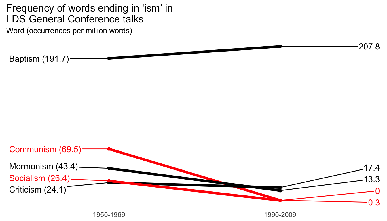
Because we saved the plot to a variable (fancy_plot), we can do stuff with it like saving it to our computer with ggsave():
ggsave(fancy_plot, filename = "output/words.pdf",
       width = 7, height = 4, units = "in")
ggsave(fancy_plot, filename = "output/words.png",
       width = 7, height = 4, units = "in")
Finally, just for fun, we can use nicer fonts to make the graphic even nicer. We’ll use Roboto Condensed, which is free from Google Fonts.
- If you’re using macOS, ensure that you install XQuartz first. That’s all you have to do to get the Cairo graphics library working.
- If you’re using Windows, either reload all the system fonts (after installing Roboto Condensed) with
extrafont::font_import()or load the Roboto Condensed fonts individually on-the-fly:
windowsFonts(`Roboto Condensed` = windowsFont("Roboto Condensed"))
windowsFonts(`Roboto Condensed Light` = windowsFont("Roboto Condensed Light"))
With that, we can specify font families and font faces (bold, italic, plain, etc.) in geom_text_repel() and in theme():
nice_fonts <- ggplot(isms_plot, aes(x = decade, y = permil, group = word, color = highlight)) +
  geom_point() +
  geom_line(size = 1.5) +
  geom_text_repel(aes(label = label_first), direction = "y", nudge_x = -1,
                  family = "Roboto Condensed Light", fontface = "plain",
                  seed = 1234) +
  geom_text_repel(aes(label = label_last), direction = "y", nudge_x = 0.3,
                  family = "Roboto Condensed Light", fontface = "plain",
                  seed = 1234) +
  scale_color_manual(values = c("black", "red")) +
  guides(color = FALSE) +
  labs(title = "Frequency of words ending in ‘ism’ in\nLDS General Conference talks",
       subtitle = "Word (occurrences per million words)",
       x = NULL, y = NULL) +
  theme_minimal(base_family = "Roboto Condensed") +
  theme(panel.grid.major = element_blank(),
        panel.grid.minor = element_blank(),
        axis.text.y = element_blank(),
        plot.title = element_text(family = "Roboto Condensed", face = "bold"),
        plot.subtitle = element_text(family = "Roboto Condensed Light",
                                     color = "grey50", face = "plain"))
nice_fonts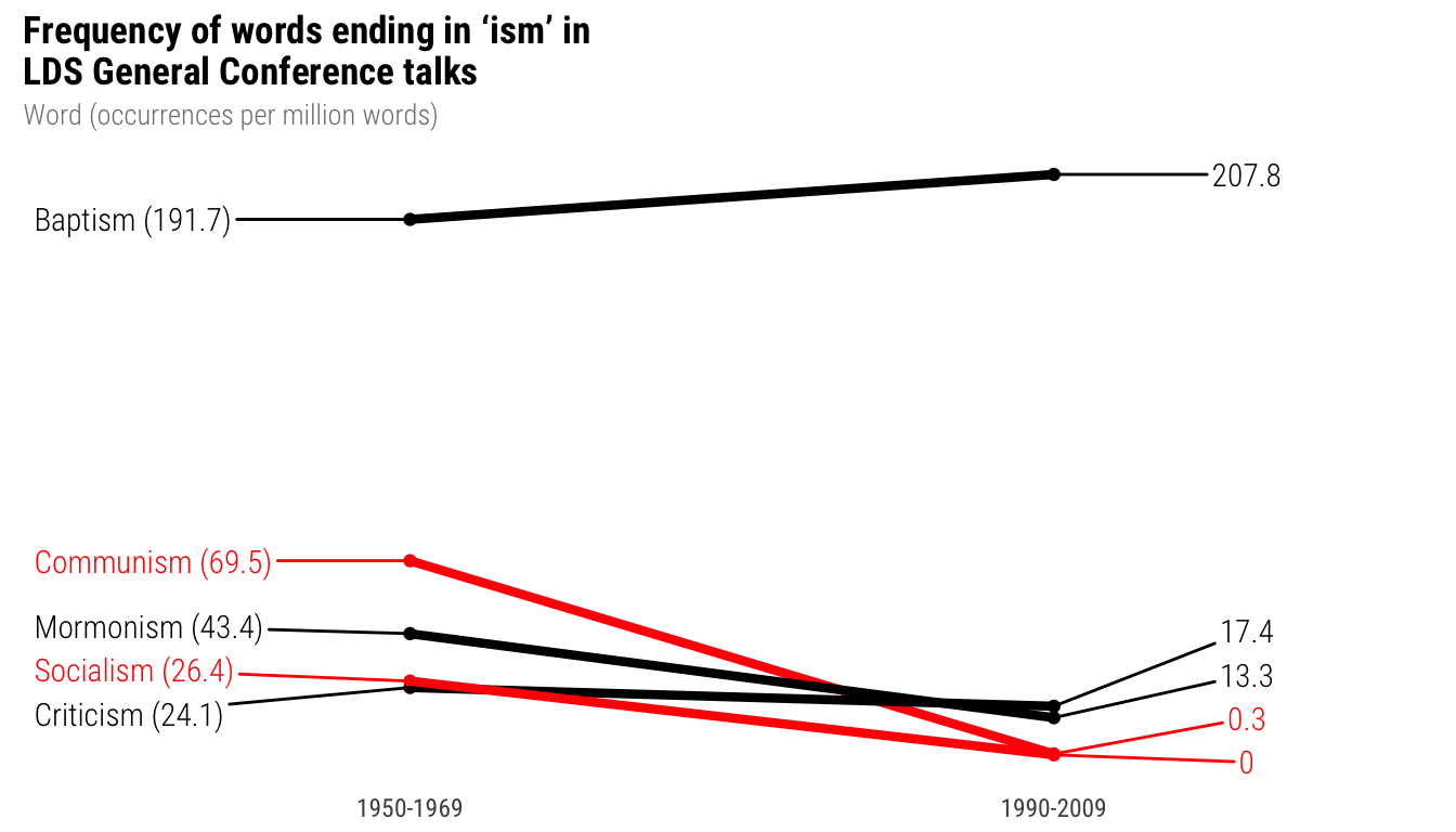
We can save the plot with the custom fonts with ggsave() like always, but we have to use the Cairo graphics library to get the fonts to embed and to get a PNG with proper dimensions. Note the difference between the two—PDFs need device = cairo_pdf while PNGs need type = "cairo". It’s different and I don’t fully understand why but ¯\_(ツ)_/¯.
ggsave(plot_isms, filename = "isms.pdf", device = cairo_pdf,
       width = 6, height = 4, units = "in")
ggsave(plot_isms, filename = "isms.png", type = "cairo",
       width = 6, height = 4, units = "in")
Bullet charts
Download fake performance data
Bullet charts are just a bunch of bar charts stacked on top of each with with extra dots and lines. First we load a data frame I copied from Stephanie Evergreen’s book, and we make sure the region variable—here named measure—is an ordered factor, and we reverse it with fct_rev() because coord_flip() does weird stuff to the ordering.
| measure | bad | satisfactory | good | target | value |
|---|---|---|---|---|---|
| Region A | 33.3 | 66.6 | 100 | 75 | 70 |
| Region B | 33.3 | 66.6 | 100 | 65 | 72 |
| Region C | 33.3 | 66.6 | 100 | 70 | 78 |
| Region D | 33.3 | 66.6 | 100 | 65 | 71 |
With the data in this form, it’s easy to plot. Here are a couple things to note:
- We overlay a bunch of
geom_col()layers with different aesthics set for each geom_errorbar()creates a line at the target level. We add ageom_point()layer in the same place for fun
ggplot(performance) +
  geom_col(aes(x = measure, y = good), fill="goldenrod2", width = 0.5, alpha = 0.2) +
  geom_col(aes(measure, satisfactory), fill="goldenrod3", width = 0.5, alpha = 0.2) +
  geom_col(aes(measure, bad), fill="goldenrod4", width = 0.5, alpha = 0.2) +
  geom_col(aes(measure, value), fill="black", width = 0.2) +
  geom_errorbar(aes(x= measure, ymin = target, ymax = target), color = "red", width = 0.45) +
  geom_point(aes(measure, target), colour = "red", size = 2.5) +
  scale_y_continuous(breaks = c(0, 50, 100)) +
  labs(x = NULL, y = NULL) +
  coord_flip() +
  theme_minimal(base_family = "Roboto Condensed") +
  theme(panel.grid.major = element_blank(),
        panel.grid.minor = element_blank())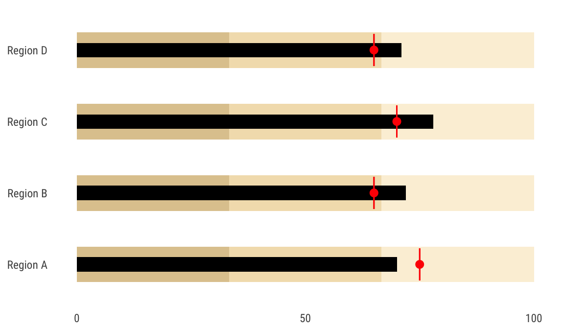
Feedback for today
Go to this form and answer these three questions (anonymously if you want):
- What new thing did you learn today?
- What was the most unclear thing about today?
- What was the most exciting thing you learned today?